SECTION 01
What is "Quant"?
At its core, quantitative finance (commonly referred to simply as "quant") is the systematic application of mathematical modeling, statistical analysis, and high-performance computing to understand financial markets, price derivatives, manage risk, and execute trades.
Beyond Gut Feeling: The Scientific Paradigm
Historically, financial trading was dominated by discretionary decision-making: portfolio managers, floor traders, and equity analysts reading corporate balance sheets, digesting macro headlines, and placing bets based on market sentiment and personal intuition.
Quantitative trading fundamentally flips this paradigm. Instead of viewing the market as an arena of human drama, quant treats it as a massive, non-stationary, and highly competitive stochastic system. Every trading strategy starts not as a hunch, but as a testable scientific hypothesis validated against rigorous historical data and deployed via automated execution algorithms.
- Relies on human intuition, narratives, and qualitative outlooks.
- Prone to cognitive biases (fear, greed, sunk-cost fallacy).
- Limited scalability across assets and microsecond timeframes.
- Difficult to systematically audit and attribute exact edge.
- Hypotheses formulated mathematically and verified statistically.
- Rule-based, automated execution completely free of emotional tilt.
- Scales seamlessly across thousands of instruments simultaneously.
- Clear statistical attribution of performance and risk factors.
The Two Engines: Smarts vs. Speed
Within modern prop trading firms and quantitative hedge funds, sustainable profitability requires the continuous synergy of two distinct pillars:
🧠
"Smarts" (Alpha & Modeling)
Markets are drowning in noise. Quants construct statistical and machine learning models to identify hidden non-linear relationships, predict price changes across varying horizons (from sub-second ticks to multi-day swings), and value complex multi-asset derivatives.
⚡
"Speed" (Low-Latency Execution)
When market events occur, multiple firms detect the opportunity simultaneously. In high-frequency electronic markets, execution is a race measured in single-digit nanoseconds. Low-latency network infrastructure, custom FPGA hardware, and kernel-bypass software ensure predictions are converted to fills before the window closes.
As industry practitioners often emphasize: "It doesn't help to be fast if you are late to realize something, and it doesn't help to be smart if your competitors capture the trade before your packets reach the matching engine."
SECTION 02
Financial Modeling & The Quant Workflow
2.1 Financial Modeling: Alpha, Beta, and the Quest for Edge
In quantitative finance, modeling is the mathematical lens used to dissect market returns. A foundational cornerstone of asset pricing theory (originating from the Capital Asset Pricing Model, or CAPM) decomposes the return of any asset or strategy into two primary forces:
$$R_i = \alpha_i + \beta_i R_m + \epsilon_i$$
β · Rm
Beta (Systematic Risk): Return driven purely by exposure to broad market movements ($R_m$).
α
Alpha (Idiosyncratic Edge): True excess return generated by active skill, independent of market direction.
ε
Epsilon (Residual Noise): Unmodeled random noise and idiosyncratic variance.
The Baseline
Beta: The Market Tide
Beta measures how strongly an asset moves with the broader market. If the S&P 500 rallies by 20% and your portfolio gains 20% simply because you held equities, that return is pure Beta.
Key Characteristic: Beta is cheap, passive, and commoditized. Anyone can buy an index ETF for a basis point of fees. However, when the market crashes 30%, Beta crashes with it.
The Holy Grail
Alpha: The Pure Edge
Alpha represents returns that cannot be explained by market beta. It is the measure of a model's ability to extract profit whether the broader market is soaring, crashing, or moving sideways.
Key Characteristic: Alpha is scarce, perishable, and zero-sum. Producing it requires sophisticated modeling, proprietary features, and relentless statistical rigor.
Why Do Quants Pursue Alpha?
Why do leading proprietary trading firms and quantitative hedge funds invest millions in compute clusters, alternative datasets, and top mathematical talent solely in pursuit of alpha?
01
All-Weather Uncorrelated Returns
Alpha strategies strive for market neutrality. Because they hedge out beta exposure ($\beta \approx 0$), they deliver high Sharpe ratios with minimal drawdowns during catastrophic market crashes.
02
Finer Margins & Scalability
Accurate predictive models allow firms to quote tighter bid-ask spreads with confidence. By anticipating where fair value is moving, quants trade at higher volume and capture margins competitors miss.
03
Defense Against Adverse Selection
In electronic order books, market makers who quote stale prices get picked off by informed traders (adverse selection). Alpha is not just an offensive weapon for profit—it is a defensive shield for survival.
2.2 $\mathbb{P}$-Quant vs. $\mathbb{Q}$-Quant: The Two Universes
Within the quantitative world, practitioners are broadly divided into two foundational paradigms named after the probability measures they inhabit: $\mathbb{P}$-Quant (the Physical or Real-World measure) and $\mathbb{Q}$-Quant (the Risk-Neutral or Martingale measure). While both share a deep mathematical foundation, their objectives, mathematical engines, tech stacks, and monetization mechanisms are radically different.
ℙ-Quant (Physical World)
The Science of Forecasting the Future
$\mathbb{P}$-quants operate in the real, objective probability space $\mathbb{P}$. Their fundamental goal is inductive prediction: analyzing historical market dynamics to estimate expected future returns $\mathbb{E}^{\mathbb{P}}[R_{t+h} \mid \mathcal{F}_t]$.
💰 How They Make Money
Directional Edge & Statistical Arbitrage: Taking calculated directional risk. They profit when an asset price moves in the direction forecasted by their statistical models (e.g., mean-reversion, momentum, cross-asset lead-lag, order book imbalance).
🛠️ Core Tech Stack & Math
Mathematics & ML
Time Series Econometrics
Gradient Boosted Trees (LightGBM)
Deep Learning (PyTorch)
Bayesian Inference
Linear Algebra
Systems & Databases
Python (Polars / NumPy)
C++ / Rust (Low Latency)
kdb+ / q (Tick DB)
ClickHouse
Ray Distributed Compute
ℚ-Quant (Risk-Neutral World)
The Science of Fair Pricing & Hedging
$\mathbb{Q}$-quants operate in an artificial risk-neutral measure $\mathbb{Q}$ where discounted asset prices are martingales. Their fundamental goal is deductive valuation: pricing a derivative contract today such that no arbitrage exists: $V_t = \mathbb{E}^{\mathbb{Q}}[e^{-r(T-t)} \Phi(S_T) \mid \mathcal{F}_t]$.
💰 How They Make Money
Spread Capture & Volatility Trading: They do not guess where the stock is going. Instead, they market-make options and derivatives, harvest bid-ask spreads, capture discrepancies between implied and realized volatility, and continuously hedge directional delta risk to stay market-neutral.
🛠️ Core Tech Stack & Math
Mathematics & Models
Itô Stochastic Calculus
Black-Scholes-Merton
Local/Stochastic Vol (SABR, Heston)
Feynman-Kac & PDEs
Girsanov Theorem
Systems & Pricing
High-Performance C++
CUDA GPU Monte Carlo
Finite Difference Solvers
QuantLib
Real-Time Greeks Engines
| Dimension |
ℙ-Quant (Physical) |
ℚ-Quant (Risk-Neutral) |
| Core Question |
"Where is the price going over horizon $h$?" |
"What is the fair price right now, and how do we replicate it?" |
| Probability Measure |
$\mathbb{P}$ (real-world empirical frequencies from historical data). |
$\mathbb{Q}$ (artificial martingale measure constructed under no-arbitrage). |
| Primary Habitat |
Proprietary statistical arbitrage firms, multi-manager hedge funds, CTA trend followers. |
Options market makers (e.g. IMC, Optiver, Citadel Securities), bank structuring and exotics desks. |
| Handling Market Risk |
Embraces directional risk: bets on favorable statistical drift. |
Eliminates directional risk: dynamically hedges delta ($\Delta \approx 0$). |
| Source of Edge |
Superior predictive modeling, feature engineering, fast reaction to novel information. |
Accurate volatility surface modeling, efficient inventory management, low-latency execution of hedges. |
⚡ The Modern Convergence: Where ℙ Meets ℚ
In leading modern electronic trading firms, the distinction between $\mathbb{P}$ and $\mathbb{Q}$ is increasingly collaborative. An options desk ($\mathbb{Q}$) relies on statistical machine learning ($\mathbb{P}$) to forecast short-term underlying drift to optimize delta hedging, while equity alpha researchers ($\mathbb{P}$) incorporate implied volatility surface skews ($\mathbb{Q}$) as forward-looking features.
2.3 The Basic Workflow of a Quant
How does an abstract idea about market dynamics transform into production code trading millions of dollars in real time? While implementations differ across firms, the standard quantitative research cycle follows a disciplined six-stage pipeline:
01
Conceptualization
Phase 1
Market Observation & Hypothesis Formulation
Contrary to popular belief, quants rarely feed blind data into black boxes. Great research starts with structural market intuition—often sparked by quant traders noticing lead-lag dynamics between an index and its heavyweight constituent, or options mispricings ahead of earnings.
Lead-Lag Dynamics
Microstructure Intuition
Trader Collaboration
02
Data Engineering
Phase 2
Data Ingestion, Cleansing & Timestamping
Financial datasets are massive and messy—often comprising tens of millions of Limit Order Book (LOB) updates per day. Quants and developers build data pipelines to reconstruct order books tick-by-tick, eliminate outliers, align nanosecond exchange timestamps, and strictly prevent lookahead or survivorship bias.
LOB Reconstruction
Nanosecond Precision
Survivorship Bias Removal
03
Signal Extraction
Phase 3
Feature Engineering & Target Formulation
Raw prices are non-stationary and non-scale-invariant. Quants transform raw quotes into meaningful predictive features: log returns, exponential moving averages (decayed returns), order flow imbalance, book skew, and cross-asset correlations. Concurrently, the prediction target and horizon (e.g. 5-minute forward return) are explicitly defined.
Decayed EMAs
Order Flow Imbalance
Horizon Calibration
04
Statistical Modeling
Phase 4
Model Formulation & Rigorous Validation
The feature matrix is passed to a statistical or machine learning model—ranging from online linear models to gradient-boosted trees and deep neural networks. The cardinal rule here is guarding against overfitting through strict walk-forward cross-validation, out-of-sample stress testing, and regularized loss functions.
Walk-Forward Validation
Regularization
Overfitting Defense
05
Execution Verification
Phase 5
Simulation & Backtesting (The Reality Check)
A model that looks stellar on paper can fail miserably in live markets if execution frictions are ignored. The simulation environment models exchange queue priority, latency penalties, market impact (the adverse price shift caused by our own order), exchange fee tiers, and risk limits.
Market Impact
Queue Priority
Slippage & Fees
06
Live Operations
Phase 6
Production Deployment & Drift Monitoring
Once validated in sim, the model is compiled into low-latency production pipelines. In live trading, quants and quant traders continuously track model parameters for distributional drift and regime shifts. When market dynamics change (such as sudden geopolitical shocks), models are refit or adjusted in real time.
Distributional Drift
Regime Detection
Trader Feedback Loop
💡 The Core Lesson of the Workflow
Quantitative research is not a linear, one-and-done project. It is a continuous, living feedback loop. As other market participants observe patterns and adapt, edge decays. Continuous innovation in feature engineering, model architecture, and execution dynamics is the lifeblood of sustained quantitative success.
SECTION 03
Methodologies & Formulations: How to Do Quant
Building a quantitative trading system requires more than economic intuition and code—it demands a rigorous mathematical formulation of the learning task. Before training a single model, a quant must rigorously define: What is the objective? What is the task format? What loss function reflects financial reality? And what mathematical tricks prevent real-world failure?
3.1 Mathematical Formulations, Tasks & Loss Functions
In financial machine learning, formulating the problem correctly is often 80% of the battle. Unlike computer vision or NLP where labels are unambiguous, financial targets are obscured by immense noise and non-stationarity.
Objectives & Loss Functions: Why Standard MSE Fails in Finance
In standard machine learning, Mean Squared Error ($\text{MSE} = \frac{1}{N}\sum (y - \hat{y})^2$) is the ubiquitous default. In quantitative finance, however, naive MSE has severe statistical and structural shortcomings:
-
✖
Fat Tails & Gradient Explosion: Financial asset returns exhibit severe leptokurtosis. A single 4-sigma flash crash squares the error, causing loss gradients to explode and models to overfit to rare, unrepeatable statistical outliers.
-
✖
The L2 vs. L1 Dilemma: Minimizing $L_2$ error (MSE) scales gradients linearly with error magnitude ($\frac{\partial L}{\partial \hat{y}} = \hat{y} - y$), warping weights to fit extreme outliers. Conversely, $L_1$ error (MAE) exerts a constant step ($\pm 1$) regardless of error size, creating a non-differentiable cusp at zero that oscillates and fails to settle near subtle signals.
-
✖
Homoskedastic Assumption: MSE assumes noise variance $\sigma^2$ is constant over time. Markets, however, exhibit extreme volatility clustering (heteroskedasticity), where errors during quiet regimes are drowned out by volatile regimes.
1. Robust Loss Functions: Huber & Log-Cosh
Huber Loss (Piecewise Quadratic / Linear):
To resolve the $L_2/L_1$ tension, Peter Huber (1964) formulated a hybrid loss: acting quadratically like $L_2$ within $[-\delta, \delta]$ for smooth convergence on subtle signals, but switching to linear $L_1$ behavior beyond $\delta$ to cap outlier gradients:
$$L_{\delta}(y, \hat{y}) = \begin{cases} \frac{1}{2}(y - \hat{y})^2 & \text{for } |y - \hat{y}| \le \delta \\ \delta\left(|y - \hat{y}| - \frac{1}{2}\delta\right) & \text{for } |y - \hat{y}| > \delta \end{cases}$$
Log-Cosh Loss (Smooth $C^\infty$ Approximation):
$$L_{\text{Log-Cosh}}(y, \hat{y}) = \sum_{i=1}^N \ln\left(\cosh(y_i - \hat{y}_i)\right)$$
Properties: A smooth, twice-differentiable ($C^\infty$) approximation to Huber loss. For small errors ($x \to 0$), $\ln \cosh x \approx \frac{x^2}{2}$ (quadratic $L_2$ like MSE). For large outliers ($|x| \to \infty$), $\ln \cosh x \approx |x| - \ln 2$ (linear $L_1$ like MAE), with continuous gradients everywhere ($\frac{\partial}{\partial \hat{y}} = -\tanh(y - \hat{y})$).
2. The Heteroskedastic Negative Log-Likelihood (NLL) Loss
To overcome the constant-variance assumption, quants predict conditional distribution parameters $(\mu_t, \sigma_t^2)$ simultaneously using the Gaussian NLL loss:
$$\mathcal{L}_{\text{NLL}}(\mu_t, \sigma_t^2) = \frac{1}{2}\ln(\sigma_t^2) + \frac{(y_t - \mu_t)^2}{2\sigma_t^2}$$
Why the log matters: The $\ln(\sigma_t^2)$ penalizes predicting infinite uncertainty, while $\frac{1}{2\sigma_t^2}$ automatically scales down prediction errors during volatile regimes—preventing regime breaks from blowing up model weights.
Where does $\sigma_t^2$ come from in practice? Quants obtain conditional variance via two primary architectures:
- Dual-Head Neural Networks (End-to-End): The model outputs two values simultaneously: predicted return $\mu_t$ and log-variance $s_t = \ln(\sigma_t^2)$. Backpropagation automatically drives $\sigma_t^2$ higher during inherently noisy, unpredictable market conditions (self-learning aleatoric uncertainty).
- Exogenous Microstructure Estimators: For tree models or linear factors, $\sigma_t^2$ is pre-calculated using high-frequency Realized Volatility ($\text{RV}_t = \sum r_{t,k}^2$), Parkinson Range Volatility ($\sigma^2 \propto \ln(H/L)^2$, 5x more efficient than close-to-close), or Implied Volatility ($\sigma_{\text{IV}}$) extracted from options surfaces.
3. The Bridge from Prediction to Capital: PnL (Profit and Loss)
In quantitative finance, statistical predictions ($\hat{y}_t$) have zero intrinsic monetary value. An asset manager cannot return prediction accuracy or low MSE to investors. The ultimate currency of all systematic trading is PnL (Profit and Loss)—the net wealth generated when portfolio allocations interact with real-world market movements.
Mathematical Formulation: Cash PnL vs. Portfolio Return ($R_{p, t}$)
For a portfolio of $N$ assets with share allocations $\mathbf{q}_{t-1} \in \mathbb{R}^N$ and price vector $\mathbf{S}_t \in \mathbb{R}^N$, the daily Cash PnL is:
$$\text{PnL}_t = \underbrace{\mathbf{q}_{t-1}^T (\mathbf{S}_t - \mathbf{S}_{t-1})}_{\text{Gross Capital Gain / Loss}} - \underbrace{\text{TC}_t}_{\text{Frictional Costs}}$$
Normalizing Cash PnL by total portfolio equity $W_{t-1}$ yields the institutional Portfolio Return $R_{p, t}$:
$$R_{p, t} = \frac{\text{PnL}_t}{W_{t-1}} = \mathbf{w}_{t-1}^T \mathbf{r}_t - \sum_{i=1}^N c_i |\Delta w_{i, t}| - \text{Borrow Costs}_t$$
Where $\mathbf{w}_{t-1} = \frac{\mathbf{q}_{t-1} \odot \mathbf{S}_{t-1}}{W_{t-1}}$ are normalized portfolio weights, $\mathbf{r}_t = \frac{\mathbf{S}_t - \mathbf{S}_{t-1}}{\mathbf{S}_{t-1}}$ are fractional asset returns, and $c_i$ represents transaction costs per unit of turnover.
The Three Critical Dimensions of Institutional PnL:
⚖️ Gross PnL vs. Net PnL
Gross PnL is frictionless paper profit at mid-market prices. Net PnL is what actually hits the fund account:
$$\text{Net PnL} = \text{Gross} - \text{Spread} - \text{Impact} - \text{Fees} - \text{Borrow}$$
Quant Reality: Novice models often claim 50%+ annual Gross returns that turn into negative Net PnL once hyperactive turnover and slippage are deducted.
📊 Realized vs. Mark-to-Market (MtM)
Realized PnL locks in cash upon trade closure. Unrealized (MtM) PnL tracks floating paper value against live market quotes:
$$\text{Total PnL}_t = \text{Realized PnL}_t + \Delta \text{Unrealized (MtM)}_t$$
Quant Reality: Prime Brokers and risk governors compute margin limits and drawdown thresholds on Mark-to-Market PnL. Traders can never conceal paper losses.
🎯 PnL Attribution & Factor Decomposition
Separates accidental market drift from authentic proprietary predictive edge:
$$\text{PnL} = \underbrace{\beta_{\text{mkt}} R_{\text{mkt}}}_{\text{Beta}} + \underbrace{\sum \beta_k f_k}_{\text{Style Factors}} + \underbrace{\alpha}_{\text{Pure Alpha}} - \text{Costs}$$
Quant Reality: Institutional LPs pay performance fees exclusively for pure Idiosyncratic Alpha PnL ($\alpha$), refusing to pay active fees for passive market beta.
The Prediction vs. PnL Disconnect: While statistical models minimize symmetric errors in price space ($\mathcal{L}_{\text{MSE}} = (\hat{y} - y)^2$), PnL is generated by positions in asymmetric decision space ($\text{PnL}_t = w(\hat{y}_t) \cdot y_t - \text{TC}_t$). A model with high win-rate or low MSE can generate devastating negative PnL if its few errors occur during volatility crashes or trigger excessive turnover.
4. The Macro Paradigm Shift: Multi-Period Compounding, Log-Utility & The Sharpe Ratio
While single-period PnL measures instantaneous cash generation ($R_{p, t} = \frac{\text{PnL}_t}{W_{t-1}}$), financial survival depends on multi-period compounding over time. This introduces a fundamental mathematical truth: wealth evolves multiplicatively, not additively.
The Log Wealth Objective: Kelly Criterion & Multi-Period Compounding
Why is the logarithm fundamental to financial optimization? Over $T$ trading periods, portfolio wealth evolves multiplicatively:
$$W_T = W_0 \prod_{t=1}^T (1 + R_{p, t}) \implies \ln\left(\frac{W_T}{W_0}\right) = \sum_{t=1}^T \ln(1 + R_{p, t})$$
Taking a second-order Taylor series expansion of $\ln(1 + R_p)$ around zero:
$$\mathbb{E}[\ln(1 + R_p)] \approx \mathbb{E}[R_p] - \frac{1}{2}\text{Var}(R_p) = \mu_p - \frac{1}{2}\sigma_p^2$$
This fundamental identity proves that maximizing expected log wealth automatically maximizes compound growth (CAGR) while heavily penalizing variance drag ($-\frac{1}{2}\sigma_p^2$). Furthermore, log-utility imposes an infinite penalty on capital wipeout: $\lim_{W \to 0} \ln(W) = -\infty$.
For a strategy with expected excess return $\mu$ and volatility $\sigma$, allocating leverage fraction $f$ yields $\mathbb{E}[\ln(1 + f R)] \approx f \mu - \frac{1}{2}f^2 \sigma^2$. Differentiating with respect to $f$ and setting to zero yields the celebrated Kelly Formula:
$$f^* = \frac{\mu}{\sigma^2} = \frac{\text{Sharpe}}{\sigma}$$
Practical Institutional Rule: Because parameter estimates $(\hat{\mu}, \hat{\sigma}^2)$ suffer from estimation error, quantitative funds almost universally trade "Half-Kelly" ($f = \frac{1}{2}f^*$)—capturing 75% of theoretical maximum growth with only 50% of the drawdown volatility.
The Operational Portfolio Metric: The Sharpe Ratio
Notice that the Kelly optimal leverage $f^* = \frac{\text{Sharpe}}{\sigma}$ directly contains the Sharpe Ratio. To operationalize log-growth across a multi-asset universe $\mathbf{w}$ while penalizing portfolio covariance $\boldsymbol{\Sigma}$, institutional finance evaluates the Sharpe Ratio as its North Star:
$$\text{Sharpe Ratio} = \frac{\mathbb{E}[R_p - R_f]}{\sigma_p} = \frac{\mathbf{w}^T \boldsymbol{\mu}}{\sqrt{\mathbf{w}^T \boldsymbol{\Sigma} \mathbf{w}}}$$
Where $\mathbf{w}$ are portfolio position weights, $\boldsymbol{\mu}$ is expected excess return, and $\boldsymbol{\Sigma}$ is the asset covariance matrix. The Sharpe ratio rewards expected return $\mathbf{w}^T \boldsymbol{\mu}$ while heavily penalizing total portfolio volatility $\sqrt{\mathbf{w}^T \boldsymbol{\Sigma} \mathbf{w}}$.
Why can a low-error regression model produce a disastrous Sharpe ratio? Three structural realities separate prediction loss from portfolio compounding:
-
✖
Symmetric Penalty on Asymmetric Windfalls: Standard regression losses penalize an asset gaining +20% when the model predicted +5% (an error of 15%) with the exact same penalty as predicting +5% when the asset crashes -10%! Investors celebrate upside volatility and penalize downside loss; point-prediction losses penalize all volatility symmetrically.
-
✖
Blindness to Portfolio Covariance ($\boldsymbol{\Sigma}$): Single-asset losses evaluate each ticker in a vacuum. They cannot detect whether predictions across 50 stocks are highly correlated, which blows up portfolio risk $\sqrt{\mathbf{w}^T \boldsymbol{\Sigma} \mathbf{w}}$.
-
✖
Ignoring Volatility Drag ($-\frac{1}{2}\sigma^2$): Standard loss functions optimize arithmetic expectations ($\mathbb{E}[R]$). But as derived above via log-expansion ($\mathbb{E}[\ln(1+R)] \approx \mu - \frac{1}{2}\sigma^2$), arithmetic gains suffer from severe volatility drag: a strategy gaining +50% followed by -50% has an arithmetic average of 0%, but destroys 25% of your actual wealth!
Empirical Simulation Experiment
The Quant Objective Paradox: Why Low MSE Loses to High Sharpe in Real Trading
504 Trading Days (2 Years) • Synthetic GARCH & Tail Shocks
To demonstrate the stark disconnect between machine learning prediction error and portfolio compounding, we simulate two systematic strategies over a 504-day trading horizon featuring regime volatility clustering and asymmetric fat-tail shocks:
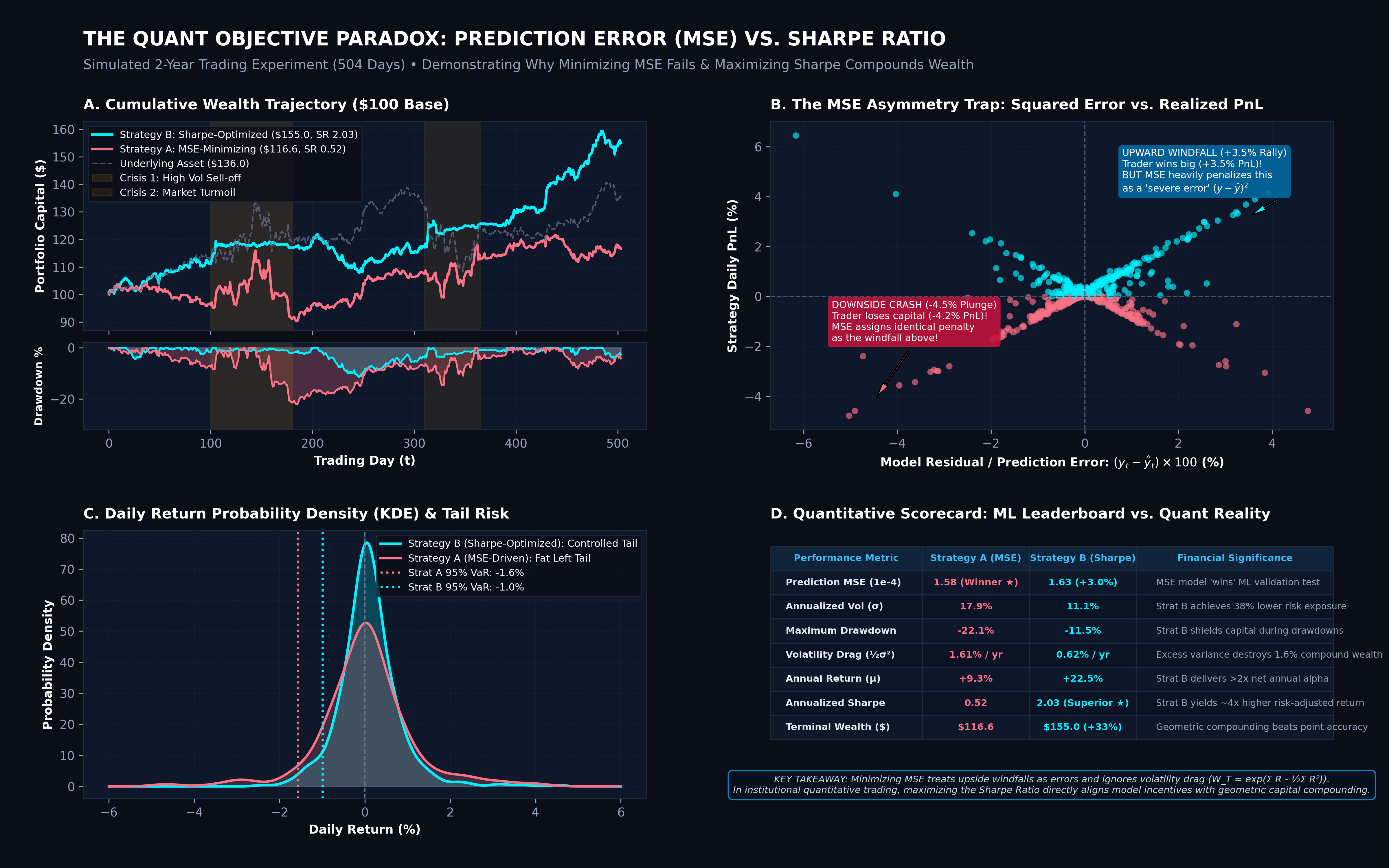
📉 Strategy A: The Naive MSE Minimizer
Achieves superior in-sample and test MSE ($1.58 \times 10^{-4}$), winning standard ML leaderboards. However, because it treats positive windfalls symmetrically with catastrophic crashes (Panel B) and sizes positions without volatility conditioning, volatility spikes induce severe drawdown (-22.1%) and volatility drag ($-\frac{1}{2}\sigma^2 = -1.61\%$/yr), ending with anemic Sharpe (0.52).
📈 Strategy B: The Sharpe-Optimized Policy
Exhibits slightly higher point prediction error ($1.63 \times 10^{-4}$, +3.0% higher MSE) because it shrinks noisy predictions. But by applying inverse-volatility Kelly sizing ($w_t \propto \frac{\hat{\mu}_t}{\hat{\sigma}_t^2}$), it compresses tail risk (Panel C), slashes volatility drag by 62%, preserves capital during market turmoil, and achieves 4x higher Sharpe (2.03) and +33% greater terminal wealth ($155.0 vs $116.6).
Takeaway for Quants: Never evaluate trading models on validation MSE alone. A model can have lower MSE while destroying capital through negative skewness and unhedged volatility drag. The true objective must penalize variance and align directly with geometric compound growth.
🎯 The North Star Metric: Information Coefficient (IC) & Grinold's Law
Rather than minimizing raw error, $\mathbb{P}$-quants evaluate signals by the Information Coefficient (IC)—the Pearson or Spearman rank correlation between predictions $\hat{y}$ and realized forward returns $y$:
$$\text{IC} = \text{corr}(\hat{y}, y), \quad \text{Rank IC} = \text{corr}(\text{rank}(\hat{y}), \text{rank}(y))$$
Why does IC matter? Because of Grinold's Fundamental Law of Active Management, which directly bridges statistical predictive power (IC) with annual portfolio Sharpe ratio / Information Ratio ($\text{IR}$):
$$\text{IR} \approx \text{IC} \times \sqrt{N}$$
Where $N$ is breadth (the number of independent trading bets per year). Even a seemingly tiny edge of $\text{IC} = 0.04$, when applied across 2,000 stocks 250 days a year ($N = 500,000$), yields extraordinary risk-adjusted profitability.
Math Deep Dive
Derivation of Grinold's Law & The Curse of Correlated Breadth
▶
Consider $N$ active investment bets with standardized forecasts $z_i \sim \mathcal{N}(0, 1)$ and true returns $r_i = \text{IC} \cdot \sigma_i \cdot z_i + \epsilon_i$, where $\epsilon_i \sim \mathcal{N}(0, \sigma_i^2(1 - \text{IC}^2))$.
Under an optimal score-weighted active portfolio with equal-volatility assets ($w_i \propto z_i$), the expected active portfolio return and active variance are:
$$\mathbb{E}[R_A] = \sum_{i=1}^N w_i \mathbb{E}[r_i] \propto N \cdot \text{IC}, \quad \text{Var}(R_A) = \sum_{i=1}^N w_i^2 \sigma_i^2 \propto N$$
Taking the ratio yields the classic Fundamental Law: $\text{IR} = \frac{\mathbb{E}[R_A]}{\sqrt{\text{Var}(R_A)}} = \text{IC} \cdot \sqrt{N}$.
⚠️ The Correlated Breadth Trap: In real markets, bets are not independent ($\rho > 0$). If $N$ assets share an average pairwise correlation $\bar{\rho}$, the effective breadth collapses according to:
$$N_{\text{eff}} = \frac{N}{1 + (N - 1)\bar{\rho}}$$
If $\bar{\rho} = 0.1$, even $N = 1,000$ assets yields an effective breadth of only $N_{\text{eff}} \approx 9.9$ independent bets! This is why quants obsess over finding orthogonal cross-asset signals rather than simply expanding universe size.
Optimization Deep Dive
Direct Policy Optimization: The Differentiable Sharpe Ratio Loss
▶
Instead of solving an intermediate regression problem ($\hat{y} \approx r$) and then running mean-variance portfolio optimization, modern deep learning architectures can optimize portfolio weights $w_t = \pi_\theta(X_t)$ directly against the Sharpe ratio over horizon $T$:
$$\mathcal{L}_{\text{Sharpe}} = - \frac{A_T}{\sqrt{B_T - A_T^2}}, \quad A_T = \frac{1}{T}\sum_{t=1}^T R_t, \quad B_T = \frac{1}{T}\sum_{t=1}^T R_t^2$$
Here $R_t = w_t^T r_t - c \|w_t - w_{t-1}\|_1$ includes transaction costs $c$. The gradient of the annualized Sharpe ratio with respect to return $R_t$ evaluates to:
$$\frac{\partial S_T}{\partial R_t} = \frac{1}{T \sigma_T} \left(1 - \frac{S_T}{2 \sigma_T^2}(R_t^2 - B_T)\right)$$
Backpropagating this gradient through a neural network directly trains the model to scale down exposure during high-volatility regimes and prioritize asymmetric trades that boost risk-adjusted return.
3.2 The Spectrum of Quant Strategies
Quantitative trading strategies are not monolithic. Across the buy-side and sell-side, quantitative methods map into four foundational families:
| Strategy Family |
Core Idea & Mechanism |
Real-World Example |
| Cross-Sectional |
Rank all universe names relative to each other at time $t$; long top predicted winners, short bottom predicted losers (market/dollar-neutral). |
Cross-sectional momentum, value, earnings quality, multi-asset factor ranking. |
| Time-Series |
Bet on an individual asset's own historical trajectory independent of peers; position sized by volatility. |
Trend following on SPX/commodities (CTA), Hurst exponent mean reversion. |
| Size / Small-Cap |
Smaller capitalization names display structural inefficiencies: liquidity discount, retail order flow dominance, and analyst neglect. |
Long small-cap / short large-cap spread, or dedicated size factor sleeves. |
| Factor / Multi-Factor |
Stack multiple weakly correlated statistical signals into an aggregated ensemble model to maximize Sharpe ratio. |
Ensemble blending: Value + Short-Term Reversal + Quality + Analyst Sentiment. |
| Event / Alternative Data |
React systematically to discrete disclosures, unstructured text, and non-traditional data streams. |
Post-Earnings Announcement Drift (PEAD), satellite oil tanker tracking, order-flow toxicity. |
💡 Method vs. Theme Clarification: Cross-Sectional is a mathematical method (ranking across an entire asset universe at a fixed timestamp). Size / Small-Cap is a factor or theme that can be implemented cross-sectionally or isolated as an independent portfolio sleeve.
| Strategy Family |
Core Idea |
The Catch / Residual Risk |
| Stat Arb / Pairs Trading |
Model cointegrated pairs or baskets; enter when the price spread diverges beyond standard deviations, betting on mean reversion. |
Correlation Breaks Structural divergence due to bankruptcies, corporate spinoffs, or regime shifts. |
| ETF / Index Arbitrage |
Exploit basis between an ETF's market price and the real-time Net Asset Value (NAV) of its underlying component basket. |
Latency & Fees Extreme competition from Tier-1 HFT firms; inventory financing and borrow friction. |
| Convertible / Merger Arb |
Exploit mispriced hybrid structures or discount spreads in corporate acquisitions. |
Deal-Break Risk Regulatory antitrust vetoes, financing collapse, or credit events. |
| Calendar / Basis Arbitrage |
Harvest spreads across futures curves (contango/backwardation roll) or crypto perpetual swap funding rates. |
Crowding & Liquidity Sudden basis blowout and forced margin liquidations during market panic. |
⚠️ The Reality of "Arbitrage": Textbook risk-free arbitrage ($P_{\text{buy}} < P_{\text{sell}}$ with zero risk) lasts microseconds and is contested by exchange co-located hardware. Virtually all real-world quantitative arbitrage is risk arbitrage: you are paid an attractive premium specifically because you warehouse residual structural risk that others want off their books.
Stat Arb Math
Cointegration, ADF Tests & The Ornstein-Uhlenbeck SDE
▶
Two asset price series $P_t^A$ and $P_t^B$ are non-stationary $I(1)$ random walks. However, if there exists a cointegrating hedge ratio $\gamma$ such that the residual spread:
$$z_t = P_t^A - \gamma P_t^B - \mu$$
is stationary $I(0)$ (verified via Augmented Dickey-Fuller test on $t$-statistic of $\Delta z_t = \rho z_{t-1} + \dots$), the spread can be modeled in continuous time as an Ornstein-Uhlenbeck (OU) mean-reverting process:
$$dz_t = -\theta(z_t - \mu) dt + \sigma dW_t$$
Where $\theta$ is the speed of mean reversion, $\mu$ is long-term equilibrium, and $W_t$ is standard Brownian motion. The half-life of mean reversion is $\tau_{1/2} = \frac{\ln 2}{\theta}$. A quant enters when $|z_t - \mu| > 2 \sigma_{OU}$ and unwinds when $z_t \to \mu$.
The Industry Debate: Is Market Making a ℙ-Quant or ℚ-Quant Strategy?
A common misconception among newcomers is that market making is strictly a ℚ-quant domain because high-profile options market makers (e.g. IMC, Optiver, Citadel Securities, Susquehanna) heavily recruit mathematical physicists to model volatility surfaces. In truth, market making spans a continuous spectrum determined by the asset class and execution latency:
Pure ℙ-Quant + Control
Cash Equities, FX & Crypto
Equities • Spot FX • Spot / Perp Crypto
No derivative contracts or risk-neutral measures exist. Quoting in limit order books (LOB) is 100% empirical ℙ-measure forecasting: predicting millisecond micro-price drift and book queue dynamics while solving Hamilton-Jacobi-Bellman (HJB) stochastic control equations to penalize inventory risk.
Classical ℚ-Quant Surface
Options & Exotic Derivatives
Index Options • Single-Stock Options • Swaptions
A single underlying stock can have over 5,000 distinct strike and maturity combinations. Quoting cannot be done on independent LOBs. Market makers calibrate arbitrage-free implied volatility surfaces under the risk-neutral measure ℚ, continuously hedging delta to isolate the volatility spread.
The ℚ × ℙ Hybrid Paradigm
Modern Electronic Options MM
HFT Options Desks • Cross-Asset Latency Desks
In modern high-frequency electronic markets, elite options market makers do not passively wait for fills. A baseline ℚ-surface sets fair value, but nanosecond ℙ-alphas from underlying futures order flow actively skew quotes or pull stale asks before informed latency arbitrageurs pick them off. Quoting is an active, directional game of adverse selection defense.
| Strategy Family |
Core Mechanism |
What You Get Paid For |
| Cash & Equity Market Making |
Provide continuous two-sided limit orders in electronic books; track the micro-price; dynamically skew quotes via inventory control to harvest the half-spread and exchange maker rebates. |
Inventory Risk Bearing price variance while holding unwanted inventory; surviving adverse selection against informed traders. |
| Options & Volatility Market Making |
Quote continuous two-sided surfaces across strikes and expiries; automatically hedge underlying delta risk; harvest structural volatility spreads and retail order flow. |
Short Gamma & Tail Risk Earning steady spread during calm regimes; suffering sudden gap risk or delta slippage during extreme volatility explosions. |
| Microstructure Alpha & Adverse Selection Defense |
Model Order Flow Imbalance (OFI), Volume-Synchronized Probability of Toxicity (VPIN), and queue priority to sniff out toxic informed flow and snipe stale quotes. |
Speed & Infrastructure Sub-microsecond FPGA / co-location execution; serving as an information filter between informed flow and noise traders. |
| Optimal Execution & Trade Scheduling |
Algorithmic liquidation of massive institutional orders into optimized child trajectories (TWAP/VWAP/POV) to trade off permanent and temporary price impact against market risk. |
Execution Efficiency Execution desks and agency algos paid for reducing transaction cost and avoiding institutional alpha erosion. |
Inventory Control
The Avellaneda-Stoikov Market Making & Inventory Skew Model
▶
How does a market maker quote bid $p^b$ and ask $p^a$ around mid-price $s$ to maximize PnL while penalizing inventory risk? The canonical Avellaneda-Stoikov model defines the market maker's reservation (indifference) price $r(s, q, t)$:
$$r(s, q, t) = s - q \gamma \sigma^2 (T - t)$$
Where $q$ is current inventory, $\gamma$ is risk aversion, $\sigma^2$ is asset volatility, and $(T - t)$ is the trading horizon.
The Intuition: When holding excess long inventory ($q > 0$), the reservation price sinks below mid-price ($r < s$). The optimal strategy shifts quotes downward: lowering the bid to stop accumulating stock, and lowering the ask to attract buyers and offload inventory. The optimal reservation-relative half-spreads are:
$$\delta^a(s, q, t) = \frac{s - r}{2} + \frac{1}{\gamma} \ln\left(1 + \frac{\gamma}{\kappa}\right), \quad \delta^b(s, q, t) = \frac{r - s}{2} + \frac{1}{\gamma} \ln\left(1 + \frac{\gamma}{\kappa}\right)$$
Total quoted spread is $\delta^a + \delta^b = \gamma \sigma^2(T - t) + \frac{2}{\gamma} \ln\left(1 + \frac{\gamma}{\kappa}\right)$, where $\kappa$ characterizes order book liquidity density ($\lambda(\delta) = A e^{-\kappa \delta}$).
Microstructure Signals
The Micro-Price, Order Flow Imbalance (OFI) & Spread Decomposition
▶
In high-frequency electronic markets, the naive mid-price $P_{\text{mid}} = \frac{P_a + P_b}{2}$ is an inadequate representation of true fair value because it treats the bid and ask as symmetric, ignoring the depth of the order queue.
1. Sasha Stoikov's Micro-Price: The volume-weighted micro-price adjusts for top-of-book volume imbalance:
$$P_{\text{micro}} = \frac{V_b P_a + V_a P_b}{V_b + V_a} = P_{\text{mid}} + \frac{V_b - V_a}{2(V_b + V_a)} (P_a - P_b)$$
When buy queue depth $V_b \gg V_a$, the imbalance ratio $I = \frac{V_b - V_a}{V_b + V_a} \to 1$, pulling $P_{\text{micro}}$ toward the ask price $P_a$, signaling an impending upward tick.
2. Order Flow Imbalance (OFI) (Cont, Kukanov & Stoikov 2014): Rather than static snapshot depth, OFI tracks the net dynamic flow of limit orders, cancellations, and market executions across discrete book updates $k$:
$$\Delta P_k \approx \frac{1}{\lambda} \text{OFI}_k + \varepsilon_k, \quad \text{where } \text{OFI}_k = \Delta V_b(t_k)\mathbb{I}_{\{\Delta P_b \ge 0\}} - \Delta V_a(t_k)\mathbb{I}_{\{\Delta P_a \le 0\}}$$
Here, $\frac{1}{\lambda}$ is Kyle's lambda measuring market depth. OFI exhibits a virtually instantaneous, linear correlation with short-term returns and serves as a premier feature in HFT alpha models.
3. Spread Decomposition & Toxic Flow: Market makers decompose quoted spread into: $\text{Spread} = \text{Handling Cost} + \text{Inventory Risk} + \text{Adverse Selection}$. They quantify adverse selection using Effective vs. Realized Spread:
$$\text{Effective Spread} = 2 D_t (P_t - M_t), \quad \text{Realized Spread}(\tau) = 2 D_t (P_t - M_{t+\tau})$$
$$\text{Price Impact / Adverse Selection}(\tau) = 2 D_t (M_{t+\tau} - M_t)$$
where $D_t \in \{+1, -1\}$ denotes trade direction. If realized spread after $\tau$ milliseconds is negative, the fill was "toxic"—the counterparty traded on superior information and the price promptly moved against the market maker.
Optimal Execution
The Almgren-Chriss Institutional Liquidation Trajectory
▶
When liquidating a large block of $Q_0$ shares over trading horizon $T$ across $N$ discrete intervals of length $\tau = T/N$, an institutional trader faces the fundamental execution trade-off: trading too rapidly creates heavy market impact, while trading too slowly incurs substantial inventory risk from asset price volatility.
Impact Decomposition: Almgren & Chriss (2000) split price impact into two independent components:
- Permanent Impact: $g(v) = \gamma v$, shifting the underlying random walk permanently: $S_k = S_{k-1} + \sigma \tau^{1/2} \xi_k - \tau \gamma v_k$.
- Temporary Impact: $h(v) = \eta v$, causing immediate execution slippage on the current trade: $\tilde{S}_k = S_{k-1} - \eta v_k$.
The Mean-Variance Objective: The trader minimizes the risk-adjusted execution cost $U = \mathbb{E}[x] + \lambda \mathbb{V}\text{ar}[x]$:
$$\mathbb{E}[x] = \frac{1}{2} \gamma Q_0^2 + \eta \sum_{k=1}^N \tau v_k^2, \quad \mathbb{V}\text{ar}[x] = \sigma^2 \sum_{k=1}^N \tau q_k^2$$
The Exact Analytical Solution: Solving the Euler-Lagrange optimality condition yields the famous hyperbolic liquidation trajectory:
$$q(t) = Q_0 \frac{\sinh(\kappa(T - t))}{\sinh(\kappa T)}, \quad \text{where Urgency Parameter } \kappa \approx \sqrt{\frac{\lambda \sigma^2}{\eta}}$$
Practical Interpretation: When risk aversion $\lambda \to 0$ (or volatility $\sigma \to 0$), $\kappa \to 0$ and the trajectory simplifies to a straight line $q(t) = Q_0(1 - t/T)$—the classical Time-Weighted Average Price (TWAP). Conversely, when urgency $\kappa$ is large, the optimal path becomes convex and heavily front-loaded, aggressively shedding shares early to insulate the fund from price drift.
| Strategy Family |
Core Idea |
What You Get Paid For |
| Vol Selling / Buying (VRP) |
Harvest the Variance Risk Premium (implied volatility typically trades at a premium over realized volatility due to crash fear). |
Tail Risk Acting as an insurance underwriter; suffering severe drawdown if sudden volatility explodes. |
| Dispersion & Correlation Arb |
Trade index options against a weighted basket of single-stock constituent options (long single vol, short index vol). |
Correlation Risk Bearing deviations between implied index correlation and realized stock correlation. |
| Structuring & Flow Desks |
Bank/dealer desks manufacture bespoke structured notes and non-linear payoff profiles requested by institutional clients. |
Margin & Skew Pocketing structural origination margin while dynamically hedging residual Greeks. |
3.3 The "Tricks of the Trade": Engineering Production Edge
Academic machine learning often assumes clean, identically and independently distributed (IID) datasets. Financial data violates every single one of these assumptions. Seasoned quants employ a suite of battle-tested engineering techniques to turn fragile academic models into robust live trading systems:
Data Sanitization
Winsorization & Robust Clipping
Raw financial returns feature extreme outliers. Quants use Median Absolute Deviation (MAD) or percentile clipping (e.g. 1st / 99th percentile) rather than standard deviation to prevent black swans from warping model gradients.
Feature Engineering
Cross-Sectional Rank Transform
Converting continuous features into uniform ranks ($[-0.5, 0.5]$ or quantiles) per timestamp. This completely eliminates macro regime drift and insulates features from broader market inflation or market-wide volatility surges.
Risk Orthogonalization
Factor & Sector Neutralization
Orthogonalizing signals against Market Beta, Sector dummies, and Size via weighted regression: $\alpha_{\text{clean}} = \alpha_{\text{raw}} - X(X^TX)^{-1}X^T \alpha_{\text{raw}}$. Ensures your PnL is pure predictive alpha rather than disguised sector exposure.
Target Formulation
Volatility Normalization of Targets
Dividing raw forward returns by realized volatility: $y_i^* = r_i / \sigma_i$. Without this trick, regression models allocate 95% of their capacity fitting high-beta volatile stocks while completely ignoring low-volatility names.
Validation Architecture
Purged & Embargoed Cross-Validation
Standard K-Fold CV creates massive lookahead leakage due to overlapping multi-period forward returns. Quants purge training samples that overlap with test labels and embargo post-test samples to respect serial auto-correlation.
Adaptive Memory
Decayed Exponential Sample Weighting
Weighting recent samples exponentially higher in the loss function: $w_t = e^{-\lambda(T - t)}$. Gives the model rapid responsiveness to shifting market regimes without discarding historical variance structures.
Objective Engineering
Cost & Turnover-Penalized Loss
Academic models optimize pure predictive accuracy, creating excessive position churn. Production models incorporate an explicit turnover and slippage penalty: $\mathcal{L}_{\text{net}} = \mathcal{L}_{\text{pred}} + \mu \sum_i |\Delta w_i| C_i$, acting as L1 shrinkage on trade churn to protect profits from broker fees.
Microstructure Alignment
Hayashi-Yoshida & Epps Alignment
At high frequencies, transactions across different assets arrive asynchronously. Standard correlation decays toward zero as sampling intervals shrink (the Epps effect). Quants employ Hayashi-Yoshida covariation estimators or tick-time volume clocks to restore true cross-asset dependency.
Linear Algebra
The Matrix Projection of Cross-Sectional Factor Neutralization
▶
Let $\boldsymbol{\alpha} \in \mathbb{R}^N$ be a vector of raw cross-sectional alpha scores for $N$ stocks. Let $\mathbf{B} \in \mathbb{R}^{N \times K}$ be the factor exposure matrix containing market beta, sector dummy indicators, and style risk factors (e.g. Barra risk models).
To purge all factor risk from $\boldsymbol{\alpha}$, we compute the orthogonal projection onto the null space of $\mathbf{B}$ using generalized least squares with market-cap weights $\mathbf{W} = \text{diag}(w_1, \dots, w_N)$:
$$\boldsymbol{\alpha}^* = \left( \mathbf{I} - \mathbf{B}(\mathbf{B}^T \mathbf{W} \mathbf{B})^{-1} \mathbf{B}^T \mathbf{W} \right) \boldsymbol{\alpha}$$
Notice that multiplying factor exposures against neutralized alpha yields exact orthogonality:
$$\mathbf{B}^T \mathbf{W} \boldsymbol{\alpha}^* = \mathbf{B}^T \mathbf{W} \left(\mathbf{I} - \mathbf{B}(\mathbf{B}^T \mathbf{W} \mathbf{B})^{-1}\mathbf{B}^T \mathbf{W}\right)\boldsymbol{\alpha} = (\mathbf{B}^T \mathbf{W} - \mathbf{B}^T \mathbf{W})\boldsymbol{\alpha} = \mathbf{0}$$
This guarantees that your portfolio's performance is driven 100% by pure idiosyncratic stock-selection skill ($\alpha$), completely immune to broader industry rotations, sector rallies, or market crashes.
SECTION 04
Evaluation, Backtesting & The Reality Gap
In quantitative finance, there is a legendary industry truism: "Every backtest is a money printer, yet most live strategies lose money."
Backtesting is the laboratory simulation where a quantitative hypothesis is tested against historical data. However, between historical simulation and live execution lies a treacherous chasm known as The Reality Gap. Overcoming this gap requires recognizing subtle statistical traps, guarding against insidious overfitting, and building models capable of surviving non-stationary market regimes.
4.1 The Backtesting Dilemma: Simulation vs. Reality
A naive backtest assumes an idealized, frictionless world where quotes are static, liquidity is infinite, and historical timestamps represent exact real-time availability. In practice, simulation models fall prey to four pervasive traps:
Trap 01
⏳ Lookahead Bias
Leaking future information into the model's historical training or execution state. Classic examples include using end-of-day closing prices to trigger 15:30 trades, training on unadjusted corporate action data, or using macroeconomic revisions published weeks after the trading date.
Trap 02
💀 Survivorship Bias
Constructing a backtest universe based on current index constituents (e.g., today's S&P 500) and running it back 10 years. This systematically ignores companies that went bankrupt, were delisted, or suffered catastrophic drawdowns (e.g., Enron, Lehman Brothers, SVB), artificially inflating performance.
Trap 03
🌊 Market Impact & Liquidity Illusion
Assuming your trade executes at the prevailing mid-quote without moving the order book. In reality, large institutional orders push the market against you. Real-world execution follows the Square-Root Law of Market Impact:
$$I \propto \sigma \cdot \sqrt{\frac{Q}{V}}$$
Where $Q$ is order size, $V$ is daily volume, and $\sigma$ is volatility. As trade size grows, impact costs swallow alpha exponentially.
Trap 04
⚡ Latency & Queue Priority
In electronic limit order books (LOBs), execution is first-in-first-out (FIFO). If a signal fires, your passive order sits at the tail of the queue. If you get filled immediately, it is frequently because an informed trader is aggressively sweeping the book—a phenomenon known as adverse selection.
4.2 The Twin Demons: Overfitting & Distributional Drift
Even if your execution pipeline is simulated with microsecond fidelity, two fundamental statistical phenomena destroy models when transitioned to production:
🧪 Overfitting & The Multiple Hypothesis Testing Curse
With modern GPU clusters, a researcher can test 50,000 parameter combinations in an afternoon. If you test 1,000 purely random Gaussian noise time-series against financial data, purely by chance ~50 will appear statistically significant at the standard $p = 0.05$ threshold.
This is known as Backtest Overfitting. In live trading, noise does not repeat itself, and the model's Sharpe ratio collapses to zero (or negative).
🏛️ The Institutional Rule: Hypothesis Pre-Registration: Top proprietary trading firms strictly forbid "blind hyperparameter exploration." Seasoned quants establish an economic or structural hypothesis upfront before writing code, and pre-register what behavior they expect out-of-sample.
In live financial markets, data generating processes are never stationary. When an alpha is discovered, competitor arbitrage gradually decays its edge. Furthermore, macroeconomic shocks, central bank policy shifts, regulatory tax amendments, or index constituent rebalancings continuously alter underlying joint distributions.
📉 1. Correlation & Beta Drift
The individual marginal distributions of feature $X$ and target $Y$ remain identical, but their correlation ($\rho / \beta$) suddenly breaks down—for instance, when an index reweights its top constituents.
🌲 2. The "Tree Model Trap"
When feature $X$ experiences mean drift into extreme uncharted territory: Tree-based models (XGBoost/LightGBM) fail catastrophically because they predict constant flat step values outside historical cuts. Linear models, while simple, extrapolate along functional slopes.
🔄 3. The Rolling Window Dilemma
Refitting online models faces an eternal trade-off: a short rolling window adapts swiftly to regime shifts but oscillates wildly with noise; a long rolling window is smooth and robust but dangerously slow to react.
4.3 Engineering Robust Evaluation: Defenses & Solutions
How do top quantitative research teams build models that maintain positive expectancy in live production? They deploy a multi-layered defense architecture:
Defense 01
🛡️ Purged & Embargoed Cross-Validation
Standard K-fold CV assumes independent samples. In finance, multi-day return labels overlap temporally. Purging removes training observations whose labels overlap with test labels. Embargoing discards a buffer of samples immediately following the test set to eliminate serial auto-correlation leakage.
Defense 02
📊 Combinatorial Purged CV (CPCV) & DSR
Developed by Marcos López de Prado, CPCV constructs all possible combinations of out-of-sample slices, generating hundreds of alternate backtested equity curves. This enables calculating the exact Probability of Backtest Overfitting (PBO) and the Deflated Sharpe Ratio (DSR), discounting performance for the number of trials attempted.
Defense 03
🔍 Change-Point Detection & Online Monitoring
Models in production run alongside statistical drift monitors (e.g., CUSUM and Page-Hinkley tests). If feature distributions drift beyond confidence intervals or prediction residuals skew systematically, automated alarms alert quants to re-estimate parameters or recalibrate target horizons.
Defense 04
🎛️ Fallback Governors & The QT/QR Pairing
During unprecedented market turmoil (e.g., unexpected tariff shocks, geopolitical flash crashes), complex models may behave erratically. In institutional production, Quant Traders step in to switch execution to simple, robust fallback models and tighten risk limits, while Quant Researchers conduct post-event forensics without knee-jerk overreactions.
🎯 The Golden Rule of Quantitative Evaluation
"A backtest is not a predictor of future returns; it is an autopsy of past assumptions." The goal of rigorous evaluation is not to produce an eye-popping historical Sharpe ratio, but to systematically falsify weak hypotheses before they risk real capital in production.
SECTION 05
Portfolio Construction & Risk Management: The Art of Staying Alive
In quantitative finance, there is a sobering market law: "Alpha gets you into the game, but risk management determines whether you survive it."
History is littered with brilliant quantitative hedge funds that collapsed not because their predictive signals were wrong, but because their portfolios were improperly sized, excessively leveraged, or betrayed by covariance breakdown—from Long-Term Capital Management in 1998 to the Quant Quake of August 2007. Converting noisy alpha forecasts into robust, tradeable portfolio weights is a mathematical discipline in its own right.
5.1 From Alpha Signals to Position Sizing: Mean-Variance Optimization
A novice quant might assume position sizing is trivial: simply allocate capital proportional to your model's predicted alpha score ($w_i \propto \alpha_i$). In institutional production, this naive approach is catastrophic: it completely ignores cross-asset correlations, concentrates risk in volatile names, and ignores market impact and turnover fees.
Modern systematic portfolio construction solves a constrained Mean-Variance Quadratic Program (QP):
$$\max_{\mathbf{w}} \; \underbrace{\mathbf{w}^T \boldsymbol{\mu}}_{\text{Expected Return}} - \underbrace{\frac{\gamma}{2} \mathbf{w}^T \boldsymbol{\Sigma} \mathbf{w}}_{\text{Variance Penalty}} - \underbrace{\lambda_{\text{cost}} \|\mathbf{w} - \mathbf{w}_0\|_1}_{\text{Turnover \& Impact Cost}}$$
$$\text{Subject to:} \quad \mathbf{w}^T \mathbf{1} = 0 \quad (\text{Dollar Neutral}), \quad \|\mathbf{w}\|_1 \le L \quad (\text{Gross Leverage Bound}), \quad w_{\min} \le w_i \le w_{\max}$$
In the unconstrained case with zero transaction costs, solving the first-order condition $\nabla_{\mathbf{w}} = \boldsymbol{\mu} - \gamma \boldsymbol{\Sigma} \mathbf{w} = \mathbf{0}$ yields the canonical analytical solution:
$$\mathbf{w}^* = \frac{1}{\gamma} \boldsymbol{\Sigma}^{-1} \boldsymbol{\mu}$$
Notice the critical operator: the inverse covariance matrix $\boldsymbol{\Sigma}^{-1}$. Inverting $\boldsymbol{\Sigma}$ is where mathematical finance crashes directly into the harsh reality of numerical instability.
5.2 The High-Dimensional Covariance Trap & Random Matrix Theory
To compute $\mathbf{w}^*$, a quant must estimate the covariance matrix $\boldsymbol{\Sigma}$ across $N$ assets. Because covariance is symmetric, this requires estimating $\frac{N(N+1)}{2}$ unique parameters. In an equity universe of $N = 500$ stocks, that requires 125,250 parameters.
If your historical estimation window covers one trading year ($T = 252$ days), the number of assets vastly exceeds the number of observations ($N > T$). In this regime, the sample covariance matrix $\mathbf{S} = \frac{1}{T}\mathbf{X}^T\mathbf{X}$ is singular, rank-deficient, and fundamentally non-invertible.
🔬 The Marchenko-Pastur Law: Why Sample Covariance Inverts Pure Noise
Even if financial returns were 100% uncorrelated Gaussian white noise, the empirical eigenvalues of $\mathbf{S}$ do not collapse to $1.0$. According to the
Marchenko-Pastur theorem (Random Matrix Theory), as $N, T \to \infty$ with ratio $q = N/T \in (0, 1)$, the empirical eigenvalues spread across a continuous spectrum bounded by:
$$\lambda_{\pm} = \sigma^2 \left(1 \pm \sqrt{q}\right)^2$$
Every eigenvalue below $\lambda_+$ is pure sampling noise! When Markowitz optimization inverts $\mathbf{S}$, the smallest noise eigenvalues ($\lambda_-$) turn into the largest inverse weights ($1/\lambda_-$). The optimizer allocates massive leveraged capital to statistical illusions.
Remedy 01
Ledoit-Wolf Optimal Shrinkage
Rather than relying on noisy empirical covariance $\mathbf{S}$, Ledoit & Wolf (2004) shrink $\mathbf{S}$ towards a structured target matrix $\mathbf{F}$ (e.g., a constant-correlation matrix): $\boldsymbol{\Sigma}^* = \delta^* \mathbf{F} + (1 - \delta^*) \mathbf{S}$. The shrinkage intensity $\delta^* \in [0, 1]$ is computed analytically to minimize expected quadratic Frobenius loss, guaranteeing positive definiteness.
Remedy 02
Hierarchical Risk Parity (HRP)
Introduced by Marcos López de Prado, HRP replaces matrix inversion with unsupervised machine learning. By computing a tree dendrogram over the correlation distance metric $d_{i,j} = \sqrt{\frac{1}{2}(1 - \rho_{i,j})}$, HRP assigns weights recursively through inverse-variance tree bifurcation. HRP requires zero matrix inversion and never blows up.
Spectral Math
Random Matrix Theory: Eigenvalue Denoising & Trace Preservation
▶
How do institutional quantitative desks denoise an empirical correlation matrix $\mathbf{C} = \mathbf{V} \boldsymbol{\Lambda} \mathbf{V}^T$?
- Compute the empirical spectral decomposition: $\boldsymbol{\Lambda} = \text{diag}(\lambda_1, \dots, \lambda_N)$ sorted in descending order.
- Calculate the theoretical Marchenko-Pastur upper bound: $\lambda_+ = \sigma^2(1 + \sqrt{N/T})^2$, where $\sigma^2 = 1 - \frac{1}{N}\sum_{\lambda_i > \lambda_+} \lambda_i$.
- Eigenvalue Clipping: All eigenvalues $\lambda_i \le \lambda_+$ represent pure sampling noise. We replace each noise eigenvalue with their average: $\bar{\lambda}_{\text{noise}} = \frac{1}{M}\sum_{i=N-M+1}^N \lambda_i$, where $M$ is the number of noise eigenvalues.
- Reconstruct the filtered correlation matrix $\mathbf{C}_{\text{clean}} = \mathbf{V} \widetilde{\boldsymbol{\Lambda}} \mathbf{V}^T$ and re-scale diagonals to exactly $1.0$.
This spectral surgery preserves the true economic factors (eigenvalues $> \lambda_+$, corresponding to the market mode and broad industry sectors) while completely neutralizing idiosyncratic noise amplification.
5.3 Structural Factor Risk Decomposition: The Barra Framework
Sophisticated quantitative funds never treat asset volatility in isolation. Under the structural factor risk framework (pioneered by Rosenberg and Barra), individual asset returns $\mathbf{r} \in \mathbb{R}^N$ are decomposed into systematic factor returns $\mathbf{f} \in \mathbb{R}^K$ and specific idiosyncratic residuals $\mathbf{u} \in \mathbb{R}^N$:
$$\mathbf{r} = \mathbf{X} \mathbf{f} + \mathbf{u}$$
where $\mathbf{X} \in \mathbb{R}^{N \times K}$ is the factor exposure matrix containing market beta, style factors (Value, Size, Momentum, Volatility, Quality), and industry sector dummies.
🏛️ Systematic Factor Risk: $\mathbf{w}^T \mathbf{X} \mathbf{F} \mathbf{X}^T \mathbf{w}$
Driven by low-dimensional factor covariance $\mathbf{F} \in \mathbb{R}^{K \times K}$ ($K \ll N$). Represents broad macro, sector, and style swings. Strict quant mandate: $\mathbf{X}^T \mathbf{w} \approx \mathbf{0}$ (Factor Neutralization).
🎯 Specific Idiosyncratic Risk: $\mathbf{w}^T \boldsymbol{\Delta} \mathbf{w}$
Driven by diagonal matrix $\boldsymbol{\Delta} = \text{diag}(\sigma_{u,1}^2, \dots, \sigma_{u,N}^2)$. Represents pure stock-specific noise. By diversifying across $N \ge 300$ stocks, idiosyncratic variance decays asymptotically as $\mathcal{O}(1/N)$.
5.4 Tail Risk & Leverage Governance
Even with a neutralized portfolio, tail events, liquidity freezes, and correlated unwinds can destroy a fund overnight. Elite quant desks enforce four non-negotiable risk barriers:
Barrier 01
VaR vs. Expected Shortfall (CVaR)
Value at Risk ($\text{VaR}_\alpha$) only reports the minimum loss at the $\alpha$-percentile, completely blind to tail severity. Quants enforce Conditional VaR (CVaR): $\text{CVaR}_\alpha = \mathbb{E}[L \mid L \ge \text{VaR}_\alpha]$, which satisfies sub-additivity and penalizes fat-tailed black swan exposures.
Barrier 02
Dynamic Volatility Targeting
Rather than maintaining static dollar exposure, quants scale portfolio leverage inversely with prevailing market volatility: $L_t = L_{\text{base}} \cdot \frac{\sigma_{\text{target}}}{\hat{\sigma}_t}$. When market volatility doubles, the system automatically cuts leverage in half, preserving capital for calmer regimes.
Barrier 03
Automated Drawdown Governors
Rigid multi-tiered circuit breakers: if peak-to-trough drawdown hits $-3\%$, new risk-taking is frozen; at $-5\%$, the OMS automatically slashes gross leverage by $50\%$; at $-8\%$, all positions are flattened to cash and strategies are locked pending post-mortem code review.
Barrier 04
Days to Liquidate (DTL) Bounds
A position that cannot be unwound during panic is an existential threat. Quants constrain position size by Average Daily Volume (ADV): $\text{DTL}_i = \frac{|w_i| \cdot \text{AUM}}{0.10 \times \text{ADV}_i} \le 2\text{ to }3\text{ days}$. No position may exceed $10\%$ of typical daily market participation.
SECTION 06
The Production Tech Stack & Execution Architecture
In academic literature, a research project concludes when an offline simulation outputs an appealing Sharpe ratio. In institutional quantitative trading, that is merely day zero.
Translating mathematical formulations into enduring profitability requires an industrial-grade engineering infrastructure capable of processing tens of millions of market events per second with sub-microsecond determinism, zero packet loss, and ironclad failover safeguards.
6.1 The Dual-Engine Reality: Python Research vs. C++/Rust Execution
Elite quantitative trading firms reject the myth of the "single-language pipeline." Instead, the architecture is intentionally bifurcated into two specialized engines optimized for radically different objective functions:
Python 3.12
Polars / Arrow
PyTorch / CUDA
ClickHouse / ArcticDB
Ray Distributed
Primary Goal: Maximizing research iteration velocity. Quants crunch terabytes of historical tick data, train deep neural networks and gradient-boosted ensembles, test alternative datasets, and run cross-sectional factor regressions. Memory allocations and interpreter overhead are acceptable because execution is asynchronous and parallelized over massive GPU clusters.
Modern C++ (20/23)
Rust
SystemVerilog (FPGA)
Solarflare EF_VI
DPDK
Primary Goal: Sub-microsecond determinism and zero tail latency. The production Order Management System (OMS) and Execution Management System (EMS) operate with zero heap allocations on hot paths (`std::pmr`), lock-free ring buffers (SPSC queues), CPU core pinning, cacheline-aligned data structures (`alignas(64)`), and kernel-bypass networking.
6.2 The Market Data Hierarchy: From L1 to Raw L3 Packet Captures
Market data is not a homogeneous stream; it exists in three distinct tiers of structural granularity. The choice of market data tier defines the maximum theoretical edge a strategy can extract:
Level 01
Top-of-Book (BBO)
Contains only the best bid, best ask, and trade prints. Ignores all depth beyond top prices.
Volume: ~1k-10k msgs/sec
Use Case: Daily/hourly factor investing, macro CTA trend-following.
Level 02
Market-by-Price (Depth)
Aggregated queue volumes across 10 to 50 discrete price levels on both bid and ask.
Volume: ~100k-500k msgs/sec
Use Case: Statistical arbitrage, institutional VWAP/TWAP, short-term momentum.
Level 03
Market-by-Order (Raw L3)
Every discrete order packet: adds, cancels, modifies, fills, with exchange order IDs and nanosecond hardware timestamps.
Volume: 10M-50M+ msgs/sec
Use Case: Market making, queue priority estimation, Order Flow Imbalance (OFI).
6.3 Event-Driven Simulation vs. Vectorized Engines
A frequent cause of strategy failure when moving from research to production is the Vectorized Backtester Trap. Vectorized backtesting applies matrix operations over historical arrays (e.g., in Polars or NumPy), assuming trades execute instantaneously at historical closing or mid prices.
In live markets, limit orders do not fill automatically just because the market price touches your limit. An institutional production backtester is an Event-Driven Discrete-Event Simulator (DES) that replicates the exact internal mechanics of an exchange matching engine:
- Queue Priority Tracking: Simulating whether the venue operates on Price-Time FIFO (e.g., NASDAQ) or Pro-Rata allocation (e.g., CME Eurodollar/Treasury futures). If 500 contracts sit ahead of you at the best bid, the simulator requires 500 aggressive sell contracts to execute before granting your order a fill.
- Cancel Race Conditions: If your alpha model triggers an order cancellation due to an incoming toxic market surge, the simulator models the network transmission flight time. If an aggressive sniper packet reaches the matching engine before your cancel packet, your order is filled at a loss.
- Market Impact Feedback: Child orders dynamically deplete simulated order book depth, widening the local spread and incurring realistic slippage.
6.4 Co-Location, Networking & The Sub-Microsecond Race
For market makers and latency arbitrageurs, the speed of light in optical fiber ($c_{\text{fiber}} \approx 200{,}000\,\text{km/s}$) is a tangible constraint. Trading servers are co-located in the same physical data centers where exchange matching engines reside:
The Quantitative Latency Spectrum
💻 CPU L1 Cache Reference
~ 1 ns
⚡ Main DRAM Memory Access
~ 50 ns
📟 FPGA Hardware Tick-to-Trade (Packet in → Out)
50 - 150 ns
🏎️ Kernel-Bypass C++ Tick-to-Trade (Solarflare EF_VI)
800 ns - 2 μs
🐢 Standard Linux OS Kernel Socket (TCP/IP stack)
15 - 30 μs
📡 Microwave Link: Chicago (Aurora CME) ↔ NJ (Secaucus NY4)
~ 4.0 ms (vs Fiber ~ 6.5 ms)
Hardware Engineering
The Anatomy of a Sub-Microsecond Tick-to-Trade Path
▶
What happens inside a state-of-the-art HFT trading server when an exchange packet arrives over a 10GbE fiber cross-connect?
- Physical Layer Ingestion (0 ns): The optical signal hits the transceiver of an Enterprise Network Interface Card (e.g., Solarflare SFN8522 or Xilinx Alveo FPGA). The hardware assigns a sub-nanosecond timestamp from an atomic PTP (IEEE 1588) clock.
- Kernel-Bypass DMA (100–300 ns): Standard operating system networking interrupts are bypassed via Solarflare EF_VI or DPDK. The Ethernet frame is transferred directly into userspace ring buffers via Direct Memory Access (DMA), avoiding all Linux kernel context switches.
- Zero-Copy Packet Parsing (300–600 ns): The C++ feed handler casts raw bytes directly onto binary packet structs (e.g. MoldUDP64 / NASDAQ ITCH 5.0) using pre-allocated memory pools.
- Alpha Evaluation & Order Generation (600–900 ns): Order book queues update via SIMD instructions. Alpha signals update, and if a trade condition triggers, an outbound order message is constructed into a binary pre-formatted buffer.
- Hardware Pre-Trade Risk Gate (900–1,050 ns): Under SEC Rule 15c3-5, orders must undergo mandatory credit and price collar checks. In ultra-low-latency architectures, this check is hardwired into an FPGA gate array in under 50 nanoseconds before blasting out the TX laser to the exchange.
Total elapsed time from market event detection to order packet departure: under 1.2 microseconds in optimized C++, and under 200 nanoseconds on pure FPGA hardware.
📚 References & Industry Sources
-
[1]
IMC Trading (2024). Quantitative Research Masterclass: Microstructure Dynamics, Alpha Modeling, and Market Making Foundations. Sydney & Global Educational Series.
-
[2]
Avellaneda, M., & Stoikov, S. (2008). High-frequency trading in a limit order book. Quantitative Finance, 8(3), 217–224.
-
[3]
Cont, R., Kukanov, A., & Stoikov, S. (2014). The Price Impact of Order Book Events. Journal of Financial Econometrics, 12(1), 47–88.
-
[4]
Almgren, R., & Chriss, N. (2000). Optimal execution of portfolio transactions. Journal of Risk, 3(2), 5–40.
-
[5]
López de Prado, M. (2018). Advances in Financial Machine Learning. John Wiley & Sons.
-
[6]
Grinold, R. C., & Kahn, R. N. (2000). Active Portfolio Management: A Quantitative Approach for Producing Superior Returns and Controlling Risk (2nd ed.). McGraw-Hill.
-
[7]
Glosten, L. R., & Milgrom, P. R. (1985). Bid, ask and transaction prices in a specialist market with heterogeneously informed traders. Journal of Financial Economics, 14(1), 71–100.
-
[8]
Markowitz, H. (1952). Portfolio Selection. The Journal of Finance, 7(1), 77–91.
-
[9]
Ledoit, O., & Wolf, M. (2004). A well-conditioned estimator for large-dimensional covariance matrices. Journal of Multivariate Analysis, 88(2), 365–411.
-
[10]
Marchenko, V. A., & Pastur, L. A. (1967). Distribution of eigenvalues for some sets of random matrices. Matematicheskii Sbornik, 72(4), 507–536.
-
[11]
López de Prado, M. (2016). Building Diversified Portfolios that Outperform Out of Sample. The Journal of Portfolio Management, 42(4), 59–69.